Profiling With Cpu Sampling And Speedscope

Mar 5th, 2021 - written by Kimserey with .

Application profiling allows developers to understand the performance and resource usage of an application. It can be used to identify hot paths or simply to explore what an application does. Today we will look at a way of capturing CPU samples for Python applications with py-spy and how to understand the resulting profiling data with speedscope.

• CPU Samples with py-spy
• Visualize Flamegraph with speedscope

CPU Samples with py-spy

There are a lot of profiling tools around but majority of them require code change. Code change means rebuilding and redeploying the application.

py-spy takes a different approach and provide profiling via capture of CPU samples by reading directly the memory of the Python program. It can sample running process by providing a pid or sample scripts. py-spy can be install via pip:

1
pip install py-spy

and for recording CPU samples we use record:

1
2
3
4
5
6
7
8
9
10
11
12
13
14
15
16
17
18
19
20
21
22
23
24
25
26
27
28
> py-spy record --help                                                             

py-spy-record 
Records stack trace information to a flamegraph, speedscope or raw file

USAGE:
    py-spy record [OPTIONS] --output <filename> --pid <pid> [python_program]...

OPTIONS:
    -p, --pid <pid>              PID of a running python program to spy on
    -o, --output <filename>      Output filename
    -f, --format <format>        Output file format [default: flamegraph]  [possible values: flamegraph, raw, speedscope]
    -d, --duration <duration>    The number of seconds to sample for [default: unlimited]
    -r, --rate <rate>            The number of samples to collect per second [default: 100]
    -s, --subprocesses           Profile subprocesses of the original process
    -F, --function               Aggregate samples by function name instead of by line number
    -g, --gil                    Only include traces that are holding on to the GIL
    -t, --threads                Show thread ids in the output
    -i, --idle                   Include stack traces for idle threads
    -n, --native                 Collect stack traces from native extensions written in Cython, C or C++
        --nonblocking            Don't pause the python process when collecting samples. Setting this option will reduce the perfomance impact of sampling, but may lead to
                                 inaccurate results
    -h, --help                   Prints help information
    -V, --version                Prints version information

ARGS:
    <python_program>...    commandline of a python program to run

Let’s start first by creating a program to demonstrate how it can be used:

1
2
3
4
5
6
7
8
9
10
11
12
13
14
15
16
17
18
19
20
21
22
23
24
25
26
"""myprogram.py"""
import time

class Hello:
    def say(self):
        time.sleep(1)
        test_three()

def test():
    hello = Hello()
    hello.say()
    time.sleep(1)
    test_three()

def test_two():
    test_three()
    test_three()

def test_three():
    time.sleep(2)

if __name__ == "__main__":
    while True:
        test()
        test_two()
        test_three()

Without looking into details of what the program does, we can extract the CPU samples from this program mb

1
2
3
4
5
> py-spy record --rate 500 --duration 30 --output profile.svg -- python3 myprogram.py

py-spy> Sampling process 500 times a second for 30 seconds. Press Control-C to exit.

py-spy> Wrote flamegraph data to 'profile.svg'. Samples: 15000 Errors: 0

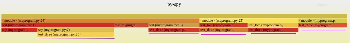
By recording the program, we get the following flamegraph:

Flamegraph allows us to see the most common code-paths and how CPU is being consumed. Here py-spy produce an icicle graph read from top to bottom, as opposed to flamegraphs which are read from bottom to top. For the rest of this post we’ll continue to refer to it as a flamegraph as it’s basically just reversed a flamegraph.

When reading a flamegraph, the following points are important to understand:

• the boxes represent functions in the stack (also refered as stack frames),
• the x-axis is the sample population - meaning the different functions - it does not represent the time passing,
• the y-axis is the depth of the stack,
• the colours do not have any meaninig, they are just used for readability purposes,
• the width of a stack frame is proportional to the time consumed by the function,
• because y-axis is the depth of the stack, the bottom line represent what is ran by the CPU,

Then from the previous flamegraph, we can start by looking at the tip of the icicles:

Highlighted with the purple bars, we find where the CPU is being used and we can easily identify test_three as a hot path. This means that any improvment on test_three would yield the highest result since it’s the function consuming about 80% (all test_three frames combined) of the CPU time.

The flamegraph also allows us to understand how the program runs, by looking at each icicle with the depth, we can deduce the following:

• <module> calls test which then call say, and say calls test_three,
• during the process of test, it also calls test_three,
• <module> calls test_twowhich then call test_three, and this happens twice,
• and <module> also directly calls test_three.

If we now compare what we read from the flamegraph, we can follow along the myprogram.py and verify that the call stack can be retraced.

So what we have seen so far is that a flamegraph allowed us to identify hot paths and understand how a program ran without prior understanding of the code.

On top of flamegraph output, py-spy also support speedscope format:

1
> py-spy record --rate 500 --duration 30 --format speedscope --output profile.speedscope.json -- python3 myprogram.py

By using --format speedscope we get a json file.

Visualize Flamegraph with speedscope

Speedscope is a web-based viewer for performance profiles. It runs smoothly on the browser and allow navigation across megabytes worth of stack frames.

We can install it locally via npm:

1
npm install -g speedscope

Then simply run speedscope to launch it.

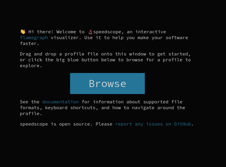
From the main page, we can upload the profile.speedscope.json that we recorded.

Speedscope provides an alternate view to flamegraph we seen earlier. Here we have access to three views:

• Time Order view which displays the frames as they were recorded in time passed order,
• Left Heavy view which displays the heavy frames on the left - this is closer to a flamegraph,
• Sandwich view which sandwiches frames between callers and callees.

Starting first by the Time Order view:

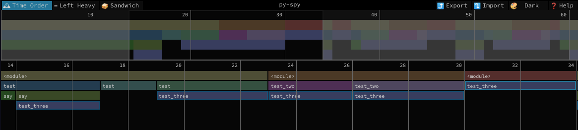
Here we can explore what was put onto the stack and how the functions were called. This is ordered by time passed hence for regular applications, it will be quite dense - but parts would be repeated as usually application paths are called again and again in the same fashion. The top timeline allows us to zoom on specific parts, we can also double click on a frame to zoom on it.

The Left Heavy view is closer to a flamegraph which does not respect the time passed but instead merge stack frames that can be merged and order them from largest to smallest from top to bottom:

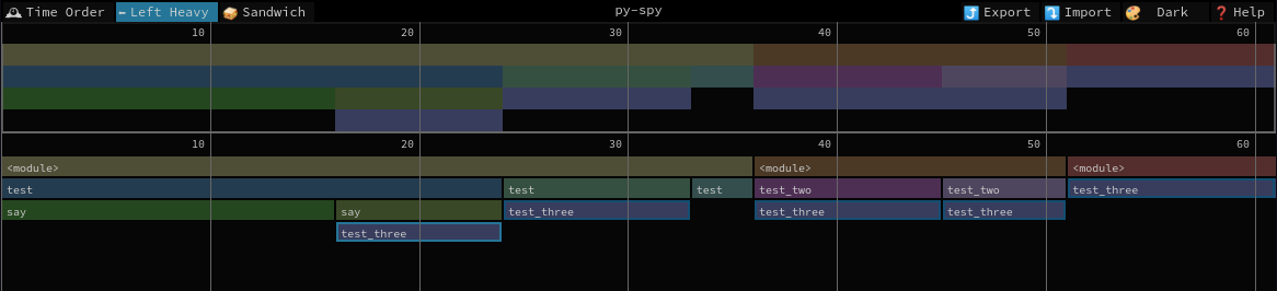
This allows use to identify quickly what frames are taking time by reading from left to right.

And lastly the Sandwich view:

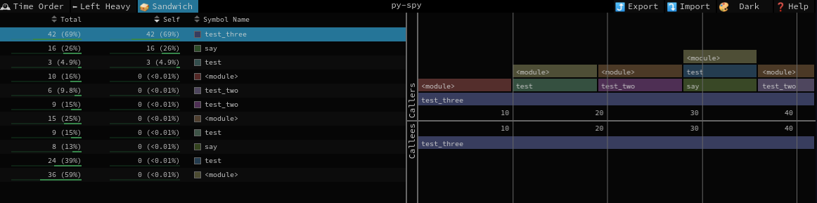
From here we can sort by time consumed for the frame itself or combined frames and when clicked on the frame we get the view of the callers and callees.

And that concludes today’s post!

Conclusion

Today we looked at how we could profile a Python application with py-spy to identify hot paths. We initially saw how we could produce and read a flamegraph using py-spy, and we then moved on to look at how the profile could also be analyzed using Speedscope, a free and open source web-based tool. I hope you liked this post and I see you on the next one!

External Sources

• Flamegraph
• PySpy Repository
• Speedscope Repository